Overview of Google's Machine Learning Crash Course - Part 1

Helps do 3 things better for Software Engineers:

Reduce time programming: Move from rule based program (logic) to writing programs where we feed it a data and we get results from it which are closer to the result.
Customize products for specific users: Ex: Instead of writing two programs for English / French users, just write a general ML program and feed it English / French to generate language specific results.
Complete unprogrammable tasks: Ex: Like computer vision / speech recognision is easier with ML than hardcoding logic.

ML changes the way a software engineer thinks from logic to statistics. More on experimentation than hardcoded logic.

Basic terminologies used in ML

Supervised Machine Learning: ML systems learn -> how to combine input -> to product useful predictions -> on never-before-seen data.

Label:

Label is a variable we are predicting. Ex: In email spam detection, a label is to identify is a mail is spam or not spam.

Typically represented by a variable y.
Features:

Features are input variables describing our data. Ex: In email spam detection, a feature might be either the contents of the email, or the sender who might be spammy.

Typically represented by a variables {x1, x2, x3, ...}

Example:

Example is a particular instance of data x. An example is a vector containing representing implicitely containing features and labels.

Examples are of two types:

 * Labelled Example:

     Has both `{features, label}: (x, y)` Ex: in email spam detection, a mail indicating where its spam or not. Maybe this input is provided by the user.

     Used to `train` a model.

 * Unlabelled Example:

     Has only `{features, ?}: (x, ?)`

     Used to make predictions (infer) on new data. Ex: A new email which our program has to detect whether spam or not based on its previous data.

Model:

A Model maps examples to predicted labels y'

The thing that is actually doing the prediction.

Two phases of a model’s life:
- Training: Training means creating or learning the model. That is, the model is shown labeled examples and enable the model to gradually learn the relationships between features and label.
- Interence: Inference means applying the trained model to unlabeled examples. That is, you use the trained model to make useful predictions (y'). Ex: During inference, a new email is predicted to be spam or not spam.

Regression: Regression model predicts continuous values. Ex: Predict housing prices, predicting probability that a user will click an advert.

Classification: Classification model predicts discrete values. Ex: Is new email spam or not spam, is image a dog or cat.

Regression

y^{'} = b + w_{'} x_{'}

Where:

y' is the predicted label (a desired output).
is the bias (the y-intercept), sometimes referred to as .
is the weight of feature 1. Weight is the same concept as the “slope” in the traditional equation of a line.
is a feature (a known input).

Loss

Loss is:

The square of the difference between the label and the prediction
  = (observation - prediction(x))2
  = (y - y')2

Simplest way to calculate loss is using Mean Square Error where Mean square error (MSE) is the average squared loss per example over the whole dataset. To calculate MSE, sum up all the squared losses for individual examples and then divide by the number of examples:

M S E = \frac{1 /}{N} \sum_{(x, y) \in D} (y - p r e d i c t i o n (x))^{2}

Although MSE is commonly-used in machine learning, it is neither the only practical loss function nor the best loss function for all circumstances.

Reducing this Loss

Training is basically to adjust the parameters going into a mathematical equation as above so that the overall loss is as low as possible

Diagram:

reducing loss

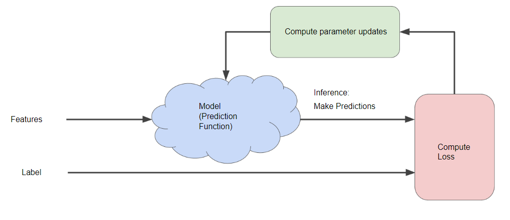
The model takes one or more features as input and returns one prediction (y') as output. To simplify, consider a model that takes one feature and returns one prediction:

y^{'} = b + w_{'} x_{'}

Starting with random initial values for b = 0 and w1 = 0 and first feature value x1 is 10, we get y' = 0.

The Compute Loss part of the diagram is the loss function that the model will use. Suppose we use the squared loss function. The loss function takes in two input values y': The model’s prediction for features x and y: The correct label corresponding to features x.

In the Compute parameter updates part of the diagram that the machine learning system examines the value of the loss function and generates new values for b and w1. Assuming this mysterious box devises new values and then the machine learning system re-evaluates all those features against all those labels, yielding a new value for the loss function, which yields new parameter values.

This continues iterating until the algorithm discovers the model parameters with the lowest possible loss. Usually, you iterate until overall loss stops changing or at least changes extremely slowly. When that happens, we say that the model has converged.

Using Gradient Descent to find the loss optimally

Compute parameter updates in diagram above is where Gradient Descent calculation is usually done.

Plotting all w1 values vs Loss:

convex

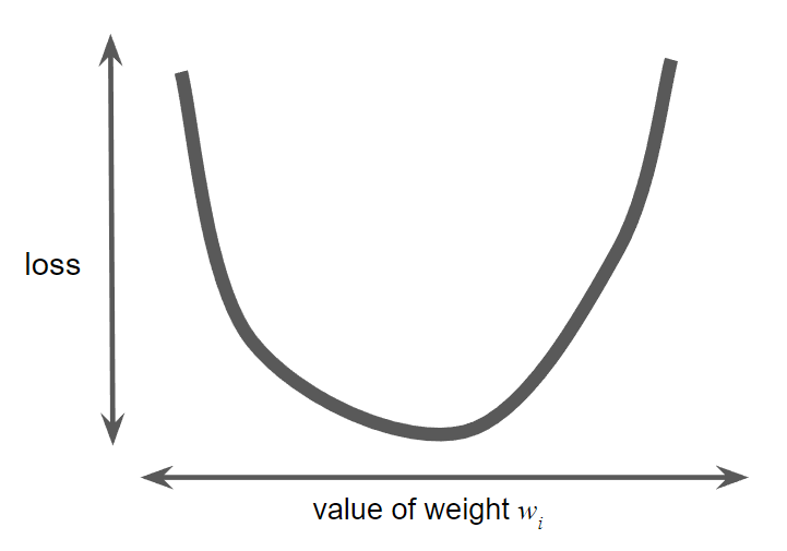
Here there is only one place where the slope is exactly 0. That minimum is where the loss function converges.

Calculating loss for all values of w1 is inefficient. This is where Gradient Descent helps.

GradientDescentGradientStep

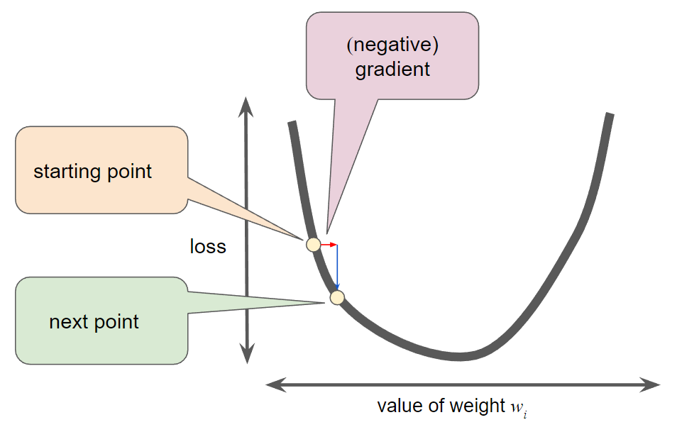
Pick some starting random value for w1 and gradient descent algorithm then calculates the gradient of the loss curve at the starting point.

The gradient of loss is equal to the derivative (slope) of the curve, and tells you which way is “warmer” or “colder.” When there are multiple weights,the gradient is a vector of partial derivatives with respect to the weights.

The gradient is vector with direction and magnitude.

The gradient always points in the direction of steepest increase in the loss function. The gradient descent algorithm takes a step in the direction of the negative gradient in order to reduce loss as quickly as possible.

Understanding the calculus behind this gradient calculation

Typically TensorFlow handles all the gradient computations. But, this section is mainly for curiosity.

Given an equation:

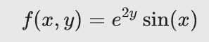
Partial derivating with y as constant:

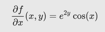
Partial derivating with x as constant:

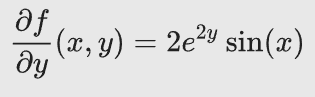
In machine learning, partial derivatives are mostly used in conjunction with the gradient of a function.

The gradient of a function, denoted as follows, is the vector of partial derivatives with respect to all of the independent variables.

Gradient for equation above:

PositiveNegativeDescent

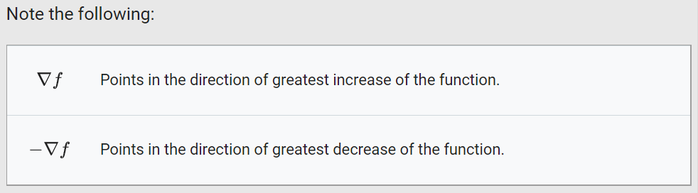
The gradient of is a two-dimensional vector that tells you in which direction to move for the maximum increase in height. Thus, the negative of the gradient moves you in the direction of maximum decrease in height. In other words, the negative of the gradient vector points into the valley which typically is lowest loss in gradient descent.

Learning Rate

Gradient descent algorithms multiply the gradient by a scalar known as the learning rate (also sometimes called step size) to determine the next point. Ex: gradient magnitude = 2.5, learning rate = 0.01, next point= 0.025.

Hyperparameters = knobs that ML engineers tweak in machine learning algorithms

Most ML engineers spend a fair amount of time tuning the learning rate cause picking small learning rate takes too much time and picking large learning rate overshoots the minima.

Goldilocks Learning rate = rate that is just right.